Cues in mass flowering of Dipterocarpaceae
Data Collection
In order to perform this analysis, I have gathered previously published flowering records at different sites throughout Southeast Asia. Table 2 below shows flowering records at each site, type of data collected, number of years the flowering was observed, and source of this data. Figure 3 shows spatial distribution of sites used in this analysis.
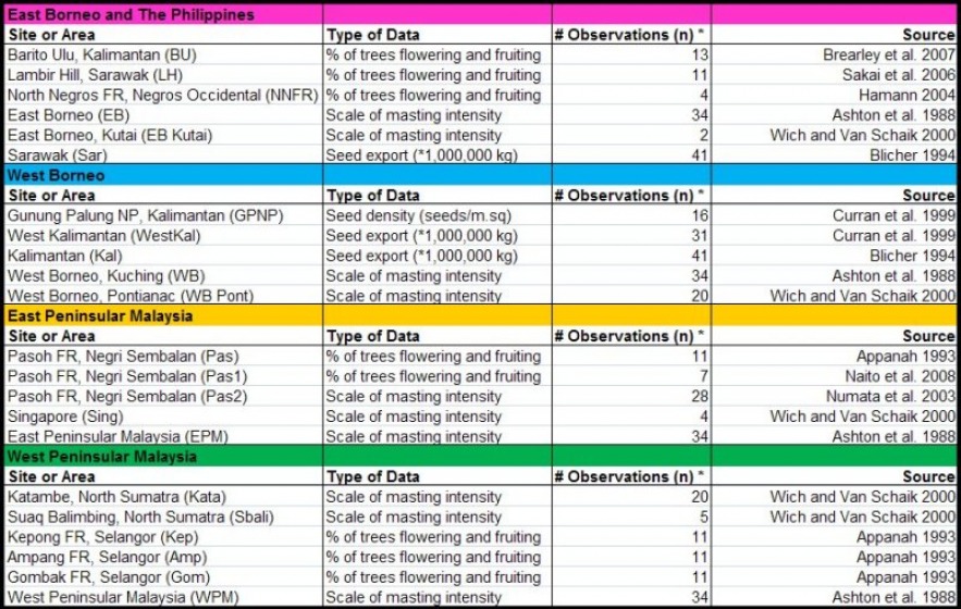
Table 2: Flowering data type and source. (* only the number of observations that are used in this analysis are noted)
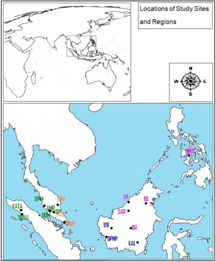
Figure 3: Map of study sites and areas.
In order to investigate a possible weather cue, I assembled relevant climate variables. Since we know from previous studies that temperature and drought seem to play a role, I chose minimum and maximum temperature measures as well as cloud cover, precipitation and humidity as indicators of drought. I also gathered various El Niño indicators (Southern Oscillation Index, Sea Surface Temperature Anomaly 3, Anomaly 3.4, and Anomaly 4). This will help in identifying areas with similar climatic cues for dipterocarp flowering in the ongoing attempt of predicting this phenomenon in the future. Table 3 below shows the compilations of all the data. Flowering data is organized on the left hand side with year, site, region and flowering intensity noted. Flowering intensity is calculated by first converting flowering data into Z scores. Z score of 1.5 and above is assigned a Mass Flowering (MF) Scale of 2. A Z score between 0.5 and 1.49 is converted to a MF Scale of 1 and anything below receives a 0. Climate and El Niño data is averaged by 'dipterocarp' years. In order to make sure that the flowering cue is included in the year when flowering occurs, weather data was averaged from October of the previous year until September of the current year. Flowering in Dipterocarpaceae starts around January/February and a flowering cue can be up to 90 days prior.
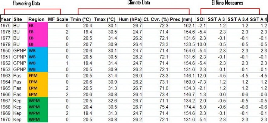
Table 3: The data table with flowering data for each site and corresponding climate and El Niño measures.
Methods
1. Clustering sites into regions that have similar weather and/or flowering patterns Using R software package ecodist.
I used Cluster analysis and Non-linear MultiDimensional Scaling (NMDS) with weather normals for study sites in order to identify specific regions of how these sites cluster. I also performed a cluster analysis with flowering observations for sites that had significant overlap of phenological data. Cluster analysis and NMDS work by converting the data table into a distance matrix that explains the similarity among observations. I used a euclidean distance measure to create a matrix for 9 weather normals for my regions (mean Annual minimum Temp., mean Annual max Temp., mean Annual Coldest Month, mean Annual Warmest Month, Mean Annual Precip., Mean Annual Cloud Cover, Mean Annual Humidity, Mean Annual Dry Season Precipitation, and Mean Annual Wet Season Precipitation). Euclidean distance measure is also known as the ordinary distance between two points identified by the Pythagorean formula. Finally, I ran a Principle Component Analysis (PCA) with correlation matrix for the weather trends and generated a biplot of the first two components. PCA works by simplifying a multivariate data table by rotating the matrix in such a way that can account for most of the variation in the data set.
2. Principle Component Analysis (PCA) and spearman's rank correlations analysis of regional weather in South East Asia
I used principle component analysis to derive weather trends based on 9 weather normals for the whole region of Southeast Asia where the study sites are located. I mapped the first three components which explain 87 % of total variance in the data set. I also ran a pearson's correlation analysis of El Niño indicators and precipitation, temperature, humidity and cloud cover in the region. I mapped the regional correlation values of sea surface temperature anomaly and all of the weather variables. The best correlation resulted with two months lag time of an onset of El Niño and weather.
3. PCA with flowering and weather correlations
Next I ran a PCA with the weather records for each site for the specific years when flowering was recorded. I used first five components, explaining 88 % total variation in the climate data, and ran a spearman's correlation with components and flowering at each one of the regions. The regions contained a groups of sites derived from the cluster and NMDS analyses from step 1. The purpose of this step is to see what components correlate well with flowering in different regions.
4. Classification and Regression Tree Analysis (CART) of flowering phenology at different sites throughout Southeast Asia
CART uses a recursive partitioning method to build classifications and regressions of the dependent variables. When the dependent variable is continuous the result is a regression tree. When the dependent variable is a class variable the result is a classification tree. I used CART to build classification trees of my flowering data (converted to presence/absence) for the regions that I have derived in step 1. I used "Rpart" package in R for this analysis.
5. Predictions of flowering using random forest
For the final part of this project, I want to see if I can use my data to predict with a degree of accuracy the onset of flowering in different regions in Southeast Asia. Random forests works by building many classification trees from your data and deciding on the best partitioning. The program later uses the training data to come up with predictions for the future based on data that you give it. In the case of this project I want to see if Random forest can predict flowering events in different regions based on the set of certain weather and El Niño indicators.
